Gradient Descent & Hill Climbing

Improving on Random Walk

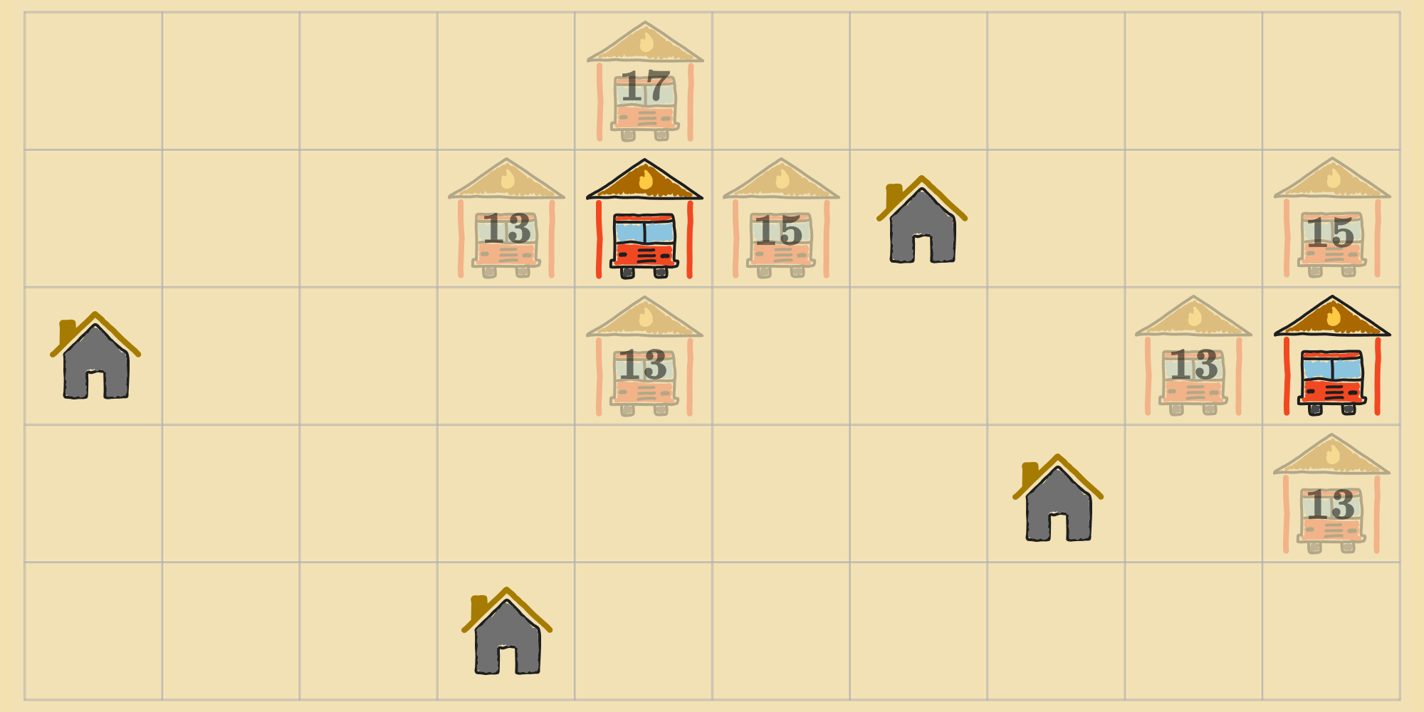
We've seen how to solve optimization problems using random walk, which is—lets be honest—a pretty dumb approach. At each step of the algorithm, because the agent is choosing actions at random, it can inefficiently stumble upon an optimal state but that doesn't guarantee that it'll find one. We can do better. Lets revisit the problem of finding the best location for two fire stations in a new town from an earlier post. Suppose this is the agent's initial state $s₀$:

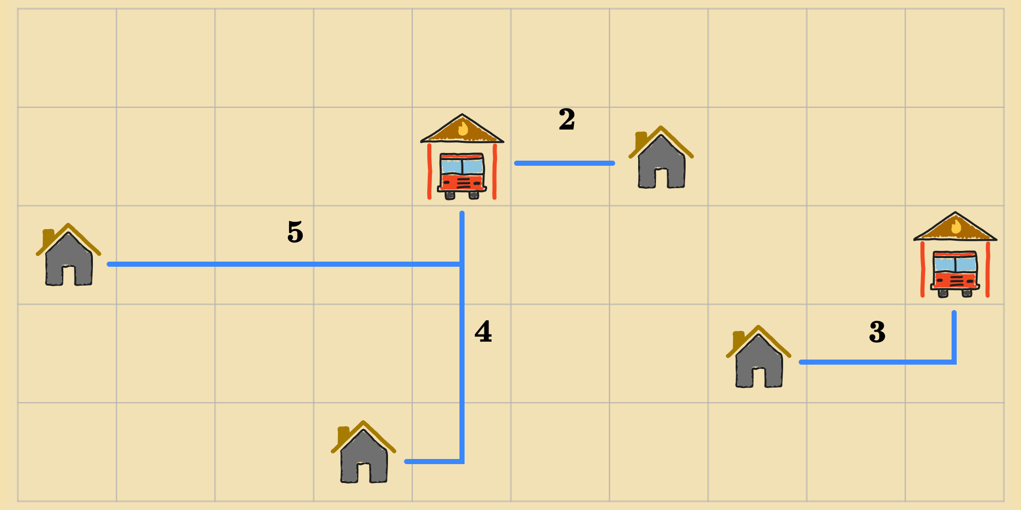
Recall that the objective function we're using for this problem is the sum of the Manhattan distances from each house to its nearest fire station. So the cost of the state in the diagram is $14$ ($= 5 + 4 + 2 + 3$). Now, the agent can choose one of the following actions ($\text{ACTIONS}(s₀)$):

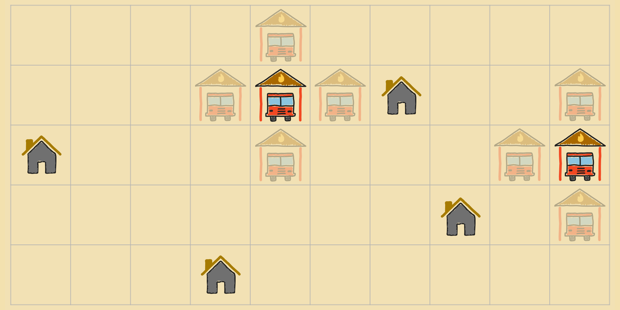
For example, the agent can shift the left-most fire station down to the cell immediately below it, or it can shift the right-most fire station left by one cell, etc. There are $7$ possible actions in total. In lieu of arbitrarily picking one of those actions to a neighboring state, the agent can calculate the cost of each of these possible successor states, i.e. $f(\text{RESULT}(s₀, a))$ for each action $a \in \text{ACTIONS}(s₀)$. So if the agent moved the left-most fire station down, that would result in the following state, with a cost of $13$ ($= 4 + 3 + 3 + 3$).

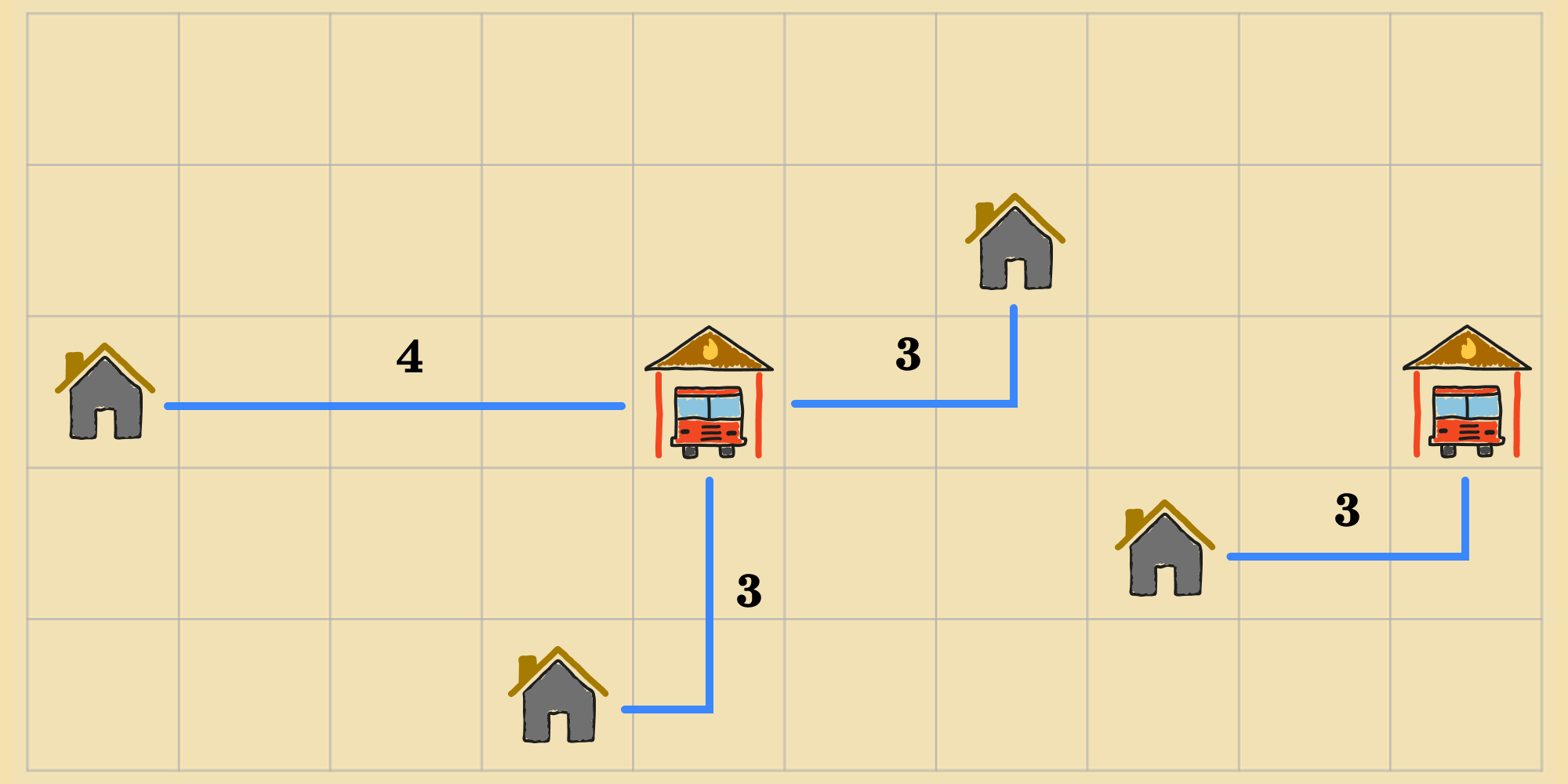
Instead, if the agent moved the right-most fire station up, that would result in this other state, with a cost of $16$ ($= 5 + 4 + 2 + 4$).

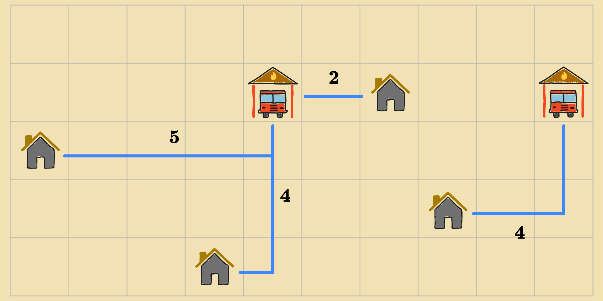
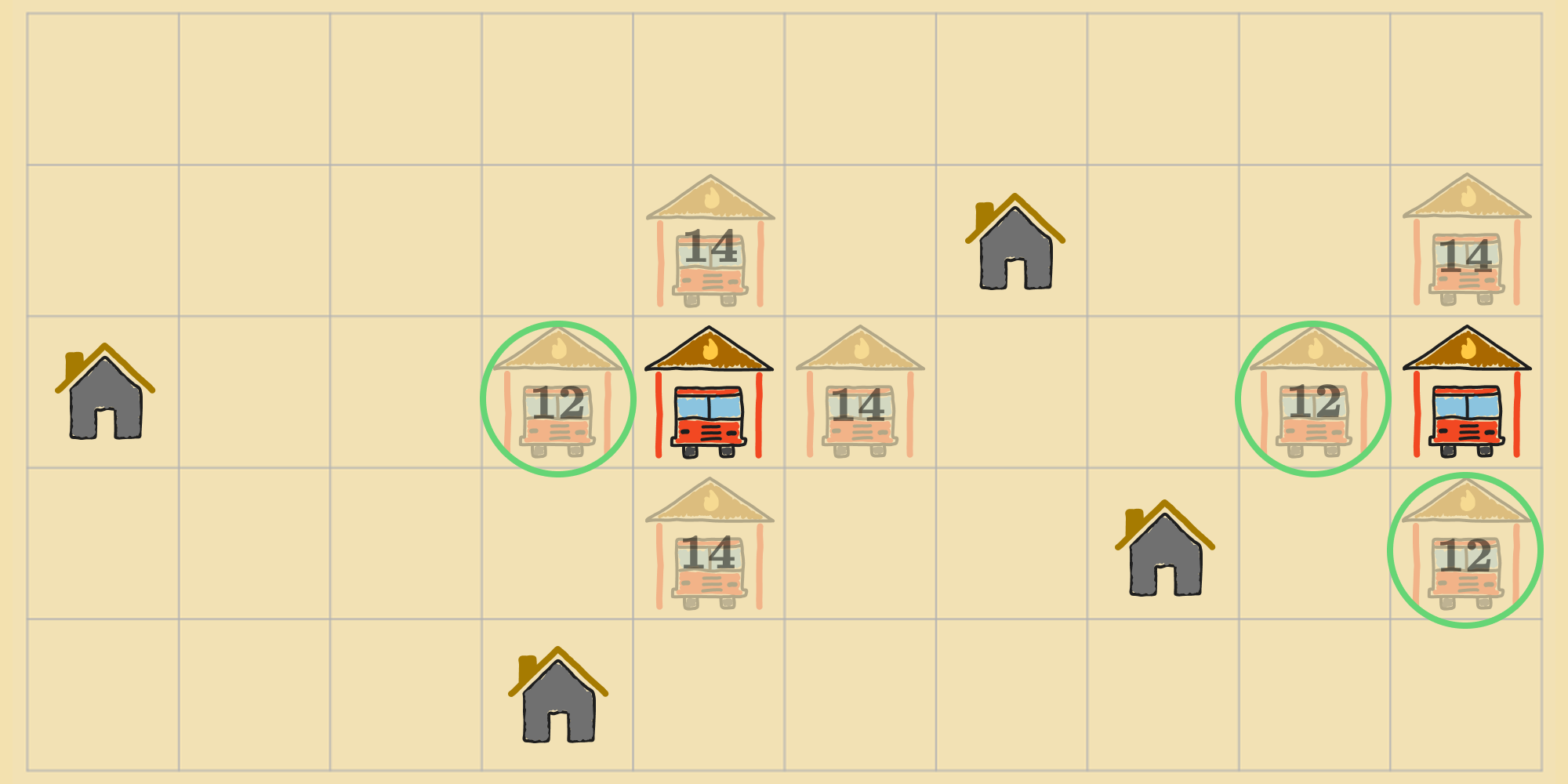
In this way, the agent can gather cost information for all of the neighbors of its current state by computing the objective function for each of the neighbors.

It can leverage this information to select the action that improves its situation the most. This means, it can select the action to the neighbor with the lowest cost. The rationale is that a state with a lower cost is probably closer to an optimal state. In this case, that would be one where the distances from each house to its closest fire station is lowest. Continuing with the example, there are $4$ neighbors with the lowest cost. The agent can transition to any one of them. Say it chooses to move the left-most fire station down by one cell.

From this new state, the agent can perform the same steps. It can compute the cost of each of the new neighboring states, and then perform the action that leads to the neighbor with the lowest cost (or any one of them if multiple neighbors are tied for lowest cost).

This way, the agent can improve the initial configuration of fire stations by moving from state to state, incrementally improving the objective function after each step. With this kind of continuous looping, we'll need a termination condition (like we did for random walk). Fortunately, there's a clear termination condition: When the agent finds itself in a state where there are no neighbors that can improve the objective function, the agent can return it's current state as the solution.

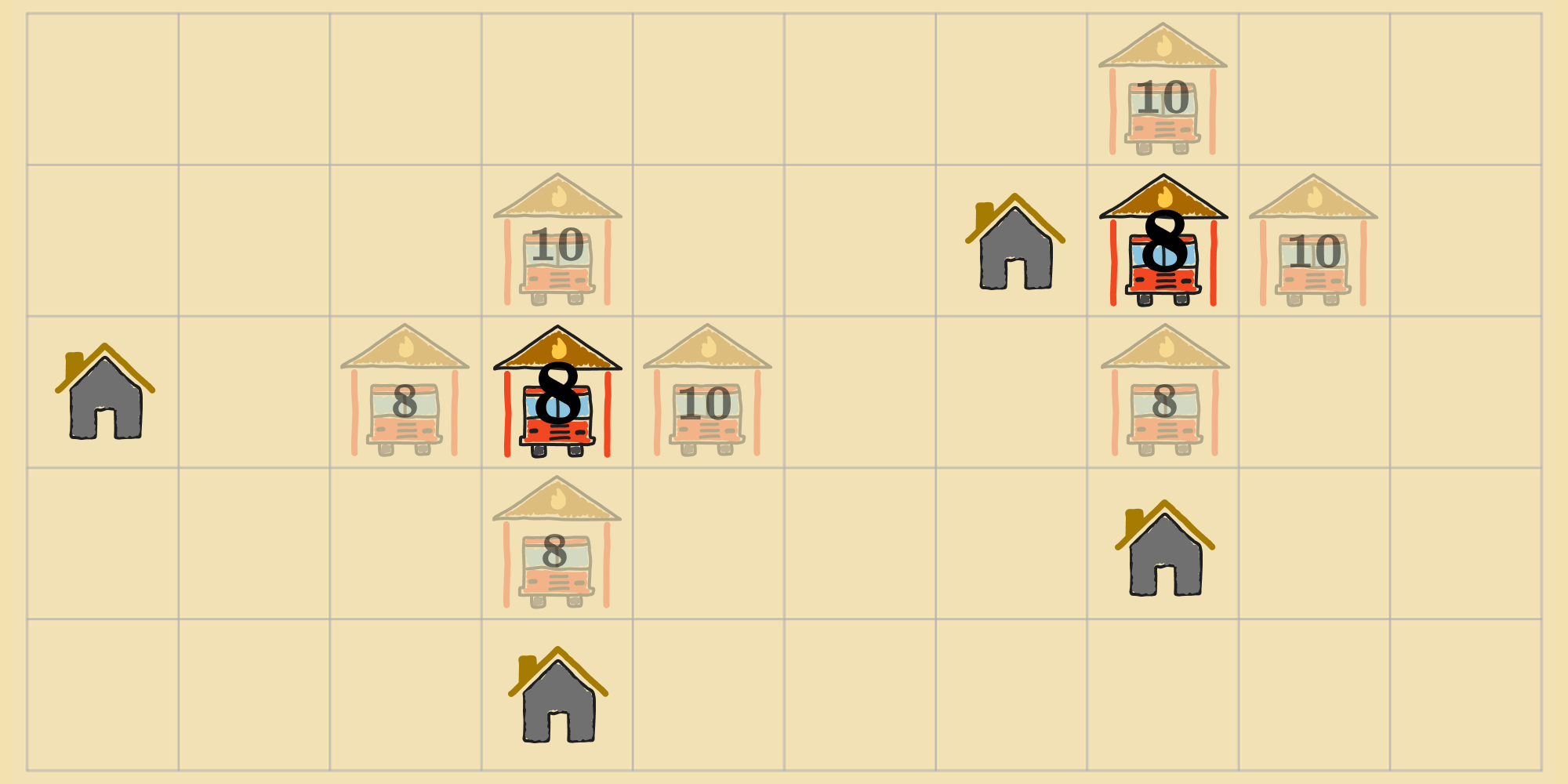
If the agent takes the left fire station and moves it up by one square, or to the right, that's going to push it further away. If the agent moves it down by one square, or the left, that doesn't change the situation: The fire station gets further away from one home, but closer to the other, on the left-side of the map. Likewise, for the other fire station, any neighbor is either going to make it further away from its nearest houses and increase the cost, or it's going to have no effect on the cost. Thus, the agent is at an optimum. This refined process of local search is known as gradient descent.

Gradient Descent - Optimizing through Greedy Choices

Gradient descent is a simple yet powerful optimization algorithm that works by iteratively moving in the direction of steepest descent of the objective function. At each state, instead of relying on randomly selecting actions, the agent evaluates the cost of each of the neighboring states according to the objective function, then transitions to the neighbor with the lowest cost, i.e. moving in the direction that most rapidly decreases the value of the objective function. It repeatedly does this—continually looking at all of the neighbors and choosing the one with the lowest value—stopping once the agent has landed in a state where none of the neighbors leads to an improvement. This state represents a minimum of the objective function.

We can formulate the algorithm for gradient descent as follows:

$$\begin{aligned} &\textbf{function}\ \text{GRADIENT-DESCENT}(s_0, f, \text{ACTIONS}, \text{RESULT}): \\ &\quad s \gets s_0 \\ &\quad \textbf{while}\ \text{true}\ \textbf{do} \\ &\quad\quad a^* \gets \arg \min_{a \in \text{ACTIONS}(s)} f(\text{RESULT}(s, a)) \\ &\quad\quad s^* \gets \text{RESULT}(s, a^*) \\ &\quad\quad \textbf{if}\ f(s^*) \ge f(s)\ \textbf{then} \\ &\quad\quad\quad \textbf{return}\ s \\ &\quad\quad \textbf{end if} \\ &\quad\quad s \gets s^* \\ &\quad \textbf{end while} \\ \end{aligned}$$

Gradient descent (and its counterpart, hill climbing, described below) is sometimes called greedy local search because it picks the best-looking neighbor state without thinking ahead about where to go next.

Hill Climbing - Searching for a Maximum

Hill climbing is the mirror image of gradient descent. Gradient descent is designed to find a minimum of an objective function through local search. But if you want to find the maximum instead, you can use hill climbing. At each iteration, instead of nudging the agent in the direction of steepest descent, it nudges in the direction of steepest ascent. It stops when the agent has reached a "peak" state, where no neighbor has a higher value. This state represents a maximum of the objective function. Figuratively, hill climbing resembles the process of trying to find the top of a mountain in a thick fog, while suffering from amnesia at the same time (i.e. not keeping track of where you've been).

$$\begin{aligned} &\textbf{function}\ \text{HILL-CLIMBING}(s_0, f, \text{ACTIONS}, \text{RESULT}): \\ &\quad s \gets s_0 \\ &\quad \textbf{while}\ \text{true}\ \textbf{do} \\ &\quad\quad a^* \gets \arg \textcolor{blue}{\max_{a \in \text{ACTIONS}(s)}} f(\text{RESULT}(s, a)) \\ &\quad\quad s^* \gets \text{RESULT}(s, a^*) \\ &\quad\quad \textbf{if}\ \textcolor{blue}{f(s^*) \le f(s)}\ \textbf{then} \\ &\quad\quad\quad \textbf{return}\ s \\ &\quad\quad \textbf{end if} \\ &\quad\quad s \gets s^* \\ &\quad \textbf{end while} \\ \end{aligned}$$

Gradient Descent in Deep Learning

Most people are familiar with gradient descent in the context of deep learning (more on that in other posts), where it's used to train neural networks. For those problems, the objective function is the loss function, and—starting from a random initialization of network weights—the goal is to iteratively improve the loss function by nudging the weights in the direction of steepest descent. This will be covered in later posts in much more detail, but we want to highlight that gradient descent is a general method, used not only in training neural networks, but—as we can see—also appropriate for many other optimization problems.