Solving Optimization Problems

From this post, introducing optimization, we can see that optimization problems closely resemble search problems, differing only in how they establish the goal. Classic search problems list the goal states $G$ explicitly, while optimization problems use the minimum or maximum value of an objective function $f$ defined over states to express the goal. So it's natural to adopt search algorithms—with some tweaks—to solving optimization problems.

Optimizing using Random Walk

As far as search algorithms go, random walk (covered in the local search post) is the most basic. We can use it for optimization just like we used it for problems like maze navigation and 8-puzzle. To see random walk in action, let's look at the fire stations' problem from the previous post:

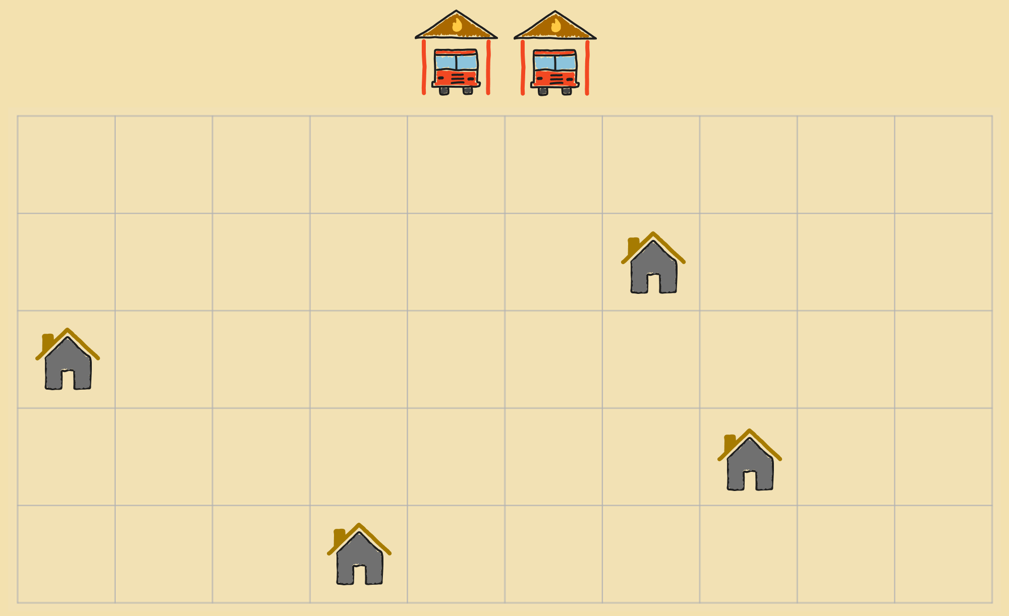
• States ($S$): The set $(x_1, y_1), (x_2, y_2)$ of all possible pairs of locations for the fire stations on the map.
• Initial State ($s₀$): The starting locations of each fire station. (Can be arbitrary.)
• Objective Function ($f$): The sum of the Manhattan distances from each house to its nearest fire station.
• Actions ($\text{ACTIONS}(s)$): Move one of the fire stations one unit in any permitted direction.
• Transition Model ($\text{RESULT}(s, a) → s'$): New state resulting from shifting one of the fire stations by one unit.

With random walk, the agent proceeds through the state space by trying a random action at each step. For example, in this state, we'd choose one of the $7$ possible moves at random.

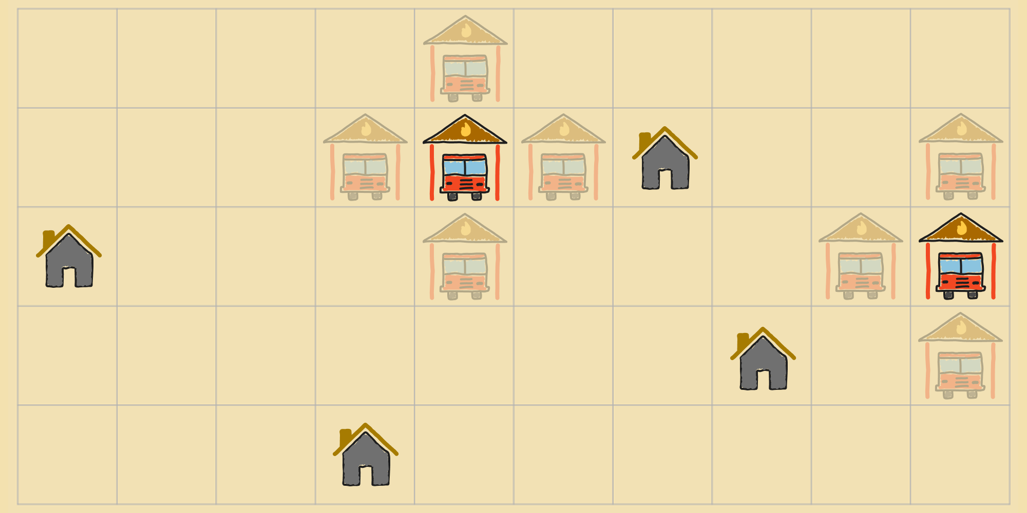
After choosing an action, the agent applies it to transition to a new state. We can repeat this process until the agent has reached a goal state. But how do we know when we've achieved the optimum, i.e. an arrangement of fire stations that minimizes the distance to each home?

As the agent is exploring the state space, we can keep track of the best state it's seen so far. If the agent arrives at a state that has a lower cost according to the objective function, then we update the best state. Once we've exhausted the state space, we return the best state as the solution. This equates to enumerating the full state space to scan for the optimal state. But this sort of brute-force search is not always possible, especially if the state space is infinite or intractably large. So instead, we can modify our random walk algorithm to terminate after a fixed amount of time (measured in steps), and return the best state the agent has encountered within that time.

$$\begin{aligned} &\textbf{function}\ \text{RANDOM-WALK}( \\ &\quad S, s_0, f, \text{ACTIONS}, \text{RESULT}, \text{MAX-ITERATIONS}): \\ &\quad s \gets s_0 \\ &\quad s_{best}, f_{best} \gets s, f(s) \\ &\quad \textbf{for}\ i \textbf{ in } [0, \text{MAX-ITERATIONS}]\ \textbf{do} \\ &\quad\quad \textbf{if}\ f(s) < f_{best}\ \textbf{then} \\ &\quad\quad\quad s_{best}, f_{best} \gets s, f(s) \\ &\quad\quad \textbf{end if} \\ &\quad\quad s \gets \text{RESULT}(s, \text{RANDOM}(\text{ACTIONS}(s))) \\ &\quad \textbf{end for} \\ &\quad \textbf{return}\ s_{best} \end{aligned}$$

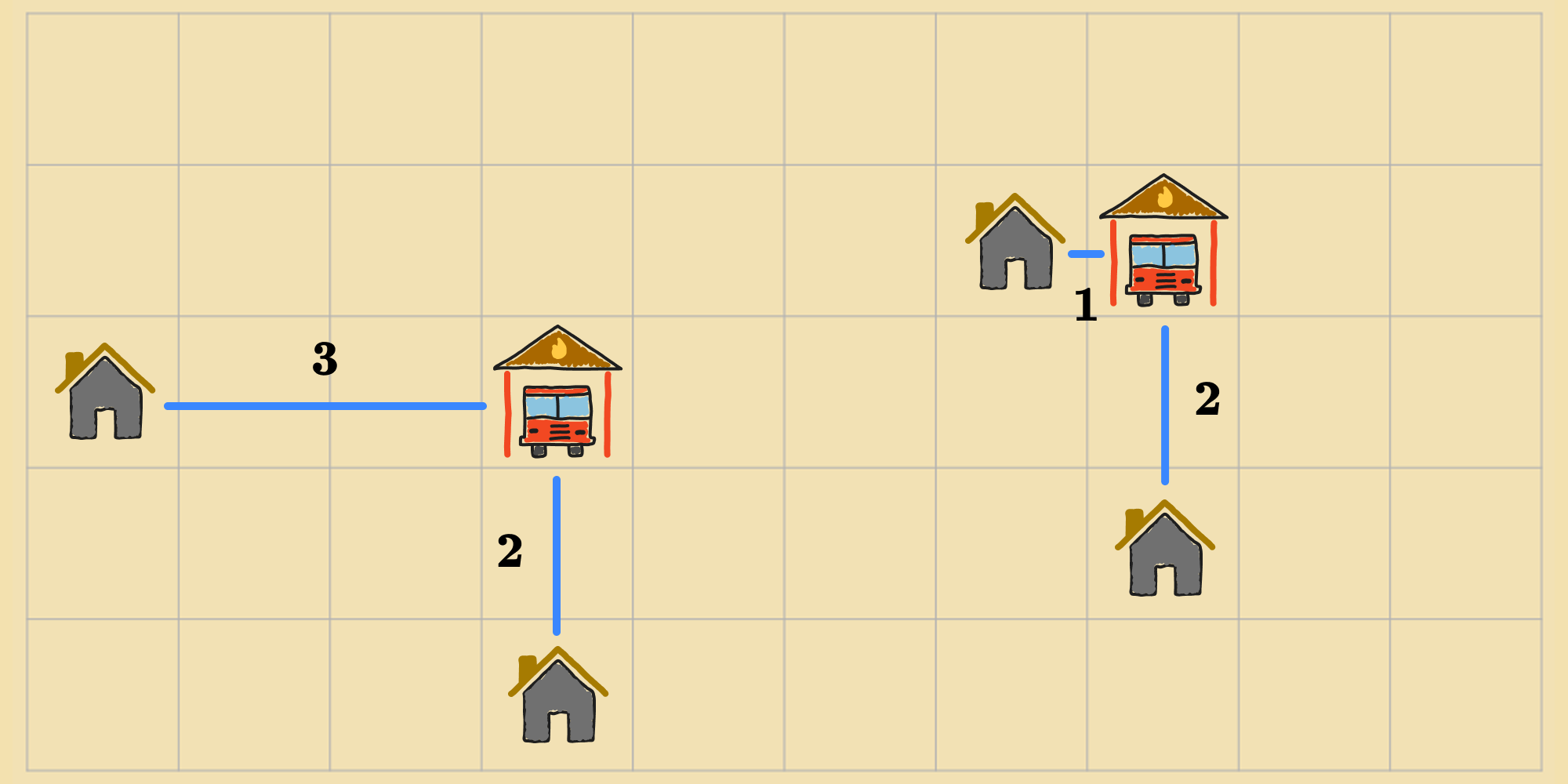
If we set $\text{MAX-ITERATIONS}$ to a large value, like $10,000$, then we'll likely reach an optimal state at some point while randomly walking (there are $|S| = \binom{46}{2} = 1,035$ possible states). Here's one solution:

Optimizing using Local Search

We can generalize our modified random walk algorithm for local search:

$$\begin{aligned} &\textbf{function}\ \text{LOCAL-SEARCH}( \\ &\quad S, s_0, f, \text{ACTIONS}, \text{RESULT}, \text{SELECTOR}, \text{MAX-ITERATIONS}): \\ &\quad s \gets s_0 \\ &\quad s_{best}, f_{best} \gets s, f(s) \\ &\quad \textbf{for}\ i \textbf{ in } [0, \text{MAX-ITERATIONS}]\ \textbf{do} \\ &\quad\quad \textbf{if}\ f(s) < f_{best}\ \textbf{then} \\ &\quad\quad\quad s_{best}, f_{best} \gets s, f(s) \\ &\quad\quad \textbf{end if} \\ &\quad\quad s \gets \text{RESULT}(s, \text{SELECTOR}(\text{ACTIONS}(s))) \\ &\quad \textbf{end for} \\ &\quad \textbf{return}\ s_{best} \end{aligned}$$

Of course, this doesn't guarantee that we'll find an optimal state that satisfies the objective function before the time limit expires, but it does allow our algorithm to terminate eventually with an acceptable solution. This may be practical in some situations, but not all.

This is a common theme with many non-analytical approaches to optimization, where a balance must be struck between accuracy and efficiency.

Optimizing using Math

Running a search-based algorithm for some optimization problems might be overkill. Some problems have closed-form solutions that can be derived mathematically. For example, if we were scouting for a location for just one fire station instead of two, and we decided to use Euclidean distance instead of Manhattan distance, we could express the objective function as:

$$f(x, y) = \sum_{i=1}^{n} \sqrt{(x_i - x)^2 + (y_i - y)^2}$$

We won't perform the derivation here, but you can deduce the closed-form solution using calculus to find the minimum of $f(x, y)$ with respect to $x$ and $y$, which would correspond to the optimal location for the fire station.

In cases where the its not possible to find a solution analytically, we may resort to search-based methods, which can be applied to a wide range of optimization problems.